Primer 1. Functions and Approximations

There is a Julia package specifically for working with Taylor series, which is apparently fast for tricky tasks. I don’t feel like I have too much to add here, but I’ll show the basic syntax of getting a Taylor series approximation of a function and plotting it, and signpost a nice video resource for getting a feeling the theory behing Taylor series.

using TaylorSeries, GLMakie
O = 5
g(x) = 2x - x^2 +x^3 +cos(x)
g_approx = taylor_expand(g, 0, order=O)

 1.0 + 2.0 t - 1.5 t² + 1.0 t³ + 0.041666666666666664 t⁴ + 𝒪(t⁶)

In Makie, we can plot a function of a single variable over a given interval as a line plot, by calling plot(interval,function).

plot(-8..8,g)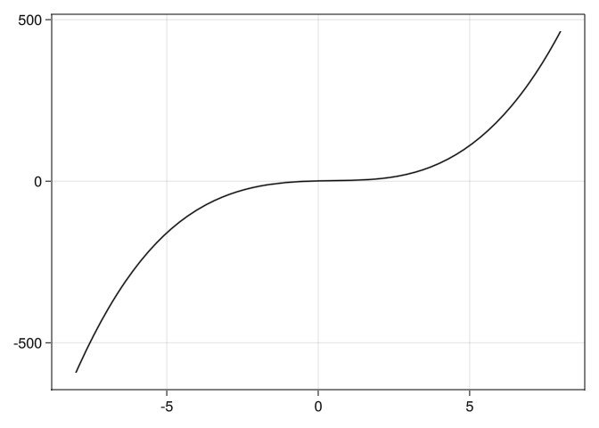

Unfortunately, we cant do plot(-8..8,g_approx) since g_approx is not a function (although it is callable confusingly enough). So if we want to use the plot(interval,function) syntax we can either create a function e.g. f(x) = g_approx(x), or we can just use an anonymous function like so.

plot!(-8..8,x -> g_approx(x))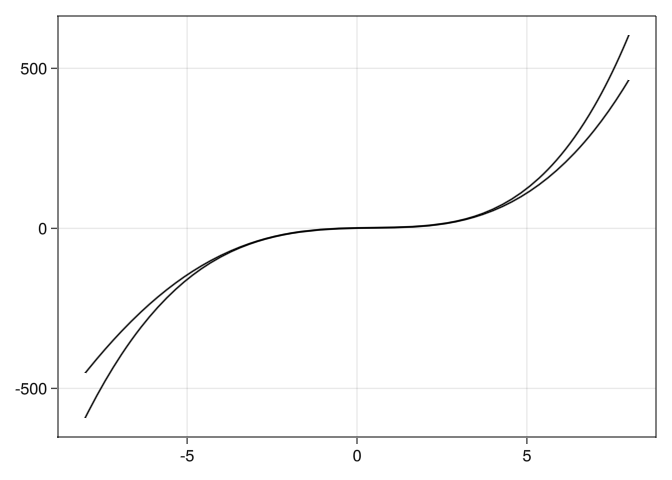

For a great video to get some intuition about how/why Taylor series approximations work, see the from Grant Sanderson.

This inspired me to try my own Taylor series animation.

using GLMakie
time = Observable(0.0)
O = Observable(0)

xs = range(-8, 8, length=80)

ys_1 = g.(xs)
prev = @lift(taylor_expand(g, 0, order=$O).(xs))
target = @lift(taylor_expand(g, 0, order=$O+1).(xs))
ys_2 = @lift($prev + ( $target - $prev) * $time)

fig = lines(xs, ys_1, color = :blue, linewidth = 4,
    axis = (title = @lift("O = $($O)"),))
lines!(xs, ys_2, color = :red, markersize = 15)

framerate = 30
timestamps = range(0, 8, step=1/framerate)
#=
record(fig, "./docs/otto_day/taylor_animation.mp4", timestamps;
        framerate = framerate) do t
    O[] = Int(floor(t))
    time[] = t -floor(t)
end
=#
pwd()

"C:\\Users\\arn203\\OneDrive - University of Exeter\\Documents\\Pages\\manual\\otto_day"

Hmmm, needs some work. Perhaps I’ll circle back round to this.